














Choosing a laser line scanner: how to calculate point spacing
To select a laser line scanner, check how many usable sampling points fall on the smallest feature at the actual profile width and working distance. Point spacing describes sampling; it is not the same as accuracy, repeatability or optical resolution.
By Michael Gold, Elina Technologies.
Two scanners can provide the same number of points per profile but very different sampling densities on the part. The difference is the width those points cover. Before comparing catalogue figures, define the feature, its tolerance and the available mounting distance.
How do you calculate point spacing within a profile?
If a profile of width W contains N uniformly spaced points, there are N − 1 intervals between the first and last point. The estimate is:
Δx ≈ W / (N − 1)
This estimates average sampling spacing. For a calibrated profile, also examine the point coordinates and local spacing around the feature. Optical calibration, a reduced measuring region, point decimation and invalid returns can change the sampling actually available.
Use the number of points in the active operating configuration, rather than automatically using the maximum catalogue value. A point rejected because of a weak return or occlusion is not a usable surface measurement.
Worked example: the same point count over different widths
Suppose the profile is 50 mm wide at the working distance and contains 1,280 points. Average spacing is 50 / 1,279 ≈ 0.0391 mm, or approximately 39.1 µm.
A 0.1 mm wide feature spans only about 2.6 sampling intervals in this example. That ratio does not prove its width can be measured to the required tolerance. Its position between samples, edge quality, optical return and the algorithm all affect the result.
| Profile width | Points per profile | Calculated average spacing |
|---|---|---|
| 25 mm | 1,280 | 19.5 µm |
| 50 mm | 1,280 | 39.1 µm |
| 100 mm | 1,280 | 78.2 µm |
| 50 mm | 2,048 | 24.4 µm |
A scanner with a narrower field can therefore provide denser sampling without a higher point count. In a real selection, the narrower field must still cover the part and its expected positional variation.
Why calculate at the actual working distance?
Line scanners have a defined measuring-field geometry. Profile width along X can change as the distance from scanner to part changes along Z. A width specified at mid-range is therefore not necessarily the width at either end of the range.
Check profile width and sampling throughout the working window the part may occupy. Do not infer both width and height range from the model name; read the measuring-field diagram for the exact model. A tilted part also requires attention to the conversion between scanner coordinates and distances along its surface.
X, Y and Z: three directions, three different questions
- X, across the laser line: point spacing within one profile affects sampling of a groove, edge or step across the line.
- Z, profile height: height linearity and repeatability are separate performance specifications. A small X spacing does not guarantee an equally small height error.
- Y, motion between profiles: 3D mapping also requires suitable spacing between successive measurement lines.
At constant motion speed v and usable profile rate f, spacing in the motion direction is Δy = v / f. For example, 200 mm/s and 2 kHz, or 2,000 profiles per second, give 0.1 mm between profiles. For variable-speed motion, check suitable synchronization, such as an encoder.
Further reading: matching measuring rate to line speed (opens in a new tab).
How many points are needed on the smallest feature?
There is no universal minimum for every measurement task. Detecting a groove, measuring its width and fitting a radius use different algorithms. Laser line width, surface slope, gloss, occlusions and data filtering also affect the result.
A target such as eight points across a feature can be a starting design assumption, but it is neither a standard nor a capability guarantee. Check usable point count and measurement error on the actual part, under production conditions and against the required tolerance. An algorithm may locate an edge between samples, but cannot guarantee recovery of details that were never measured.
How to select a laser line scanner in practice
- Define the measurement: width, height, angle, presence or profile, including the smallest feature and its tolerance.
- Establish the mounting distance and working window, and check that the part remains within the measuring field.
- Estimate X spacing and inspect local sampling and valid points around the feature.
- Check Z linearity and repeatability separately, together with profile rate and Y spacing.
- Validate using representative parts, including the most difficult expected surface and production conditions.
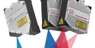
Start with 2D/3D laser profile sensors (opens in a new tab) and consider the Micro-Epsilon scanCONTROL family (opens in a new tab). Suitability depends on the model and configuration, not the family name alone.
Frequently asked questions about laser scanner point spacing
Do more points per profile always give a better measurement?
No. Compare profile width at the working distance, return quality, usable data and the algorithm. A large point count over a wide field can produce larger spacing than a smaller point count over a narrow field.
Is point spacing the same as X resolution or accuracy?
Point spacing describes sampling density across a profile. A manufacturer may also use “X resolution” to mean point count, so check its definition. Do not automatically equate it with accuracy, repeatability or optical resolving capability.
Why divide by the number of points minus one?
When N uniformly spaced points include both ends of width W, there are N − 1 intervals between them. That is the calculation assumption. For calibrated or nonuniform sampling, also check the actual X coordinates and the manufacturer’s definition.
Do eight points across a feature guarantee it can be measured?
No. This can be a planning target, but there is no universal rule. Capability depends on the task, tolerance, valid points, surface and algorithm, and must be tested under operating conditions.
What is needed for an application assessment?
Production-condition sample parts, a drawing with dimensions and tolerances, the smallest feature, mounting distance, working window, motion speed and required cycle time.
Sources and further reading
This explanation is based on Michael Gold’s article and measurement principles described in the manufacturer documentation. The numerical examples are illustrative calculations, not product performance tests.
- Micro-Epsilon scanCONTROL 30xx manual: measurement principle and technical data (opens in a new tab).
- Micro-Epsilon Configuration Tools: points per profile, measuring field and profile rate (opens in a new tab).
- Micro-Epsilon: calibrated profiles for software integration (opens in a new tab).
- Laser triangulation on shiny surfaces (opens in a new tab).
Need to select a scanner for your part? Contact the Elina team (opens in a new tab) with the application details to assess a suitable configuration.